What are trees?
Trees are a type of non-linear data structure. This means that elements are not stored sequentially. When compared against linear data structures such as linked lists or arrays, this property implies that all elements cannot be traversed in a ‘single run’ - linked lists allow all elements to be reached by just calling each node’s child, where trees do not. However, this non-linear structure does provide several advantages that will be discussed. General structure and terminology related to trees is covered by the below diagram:
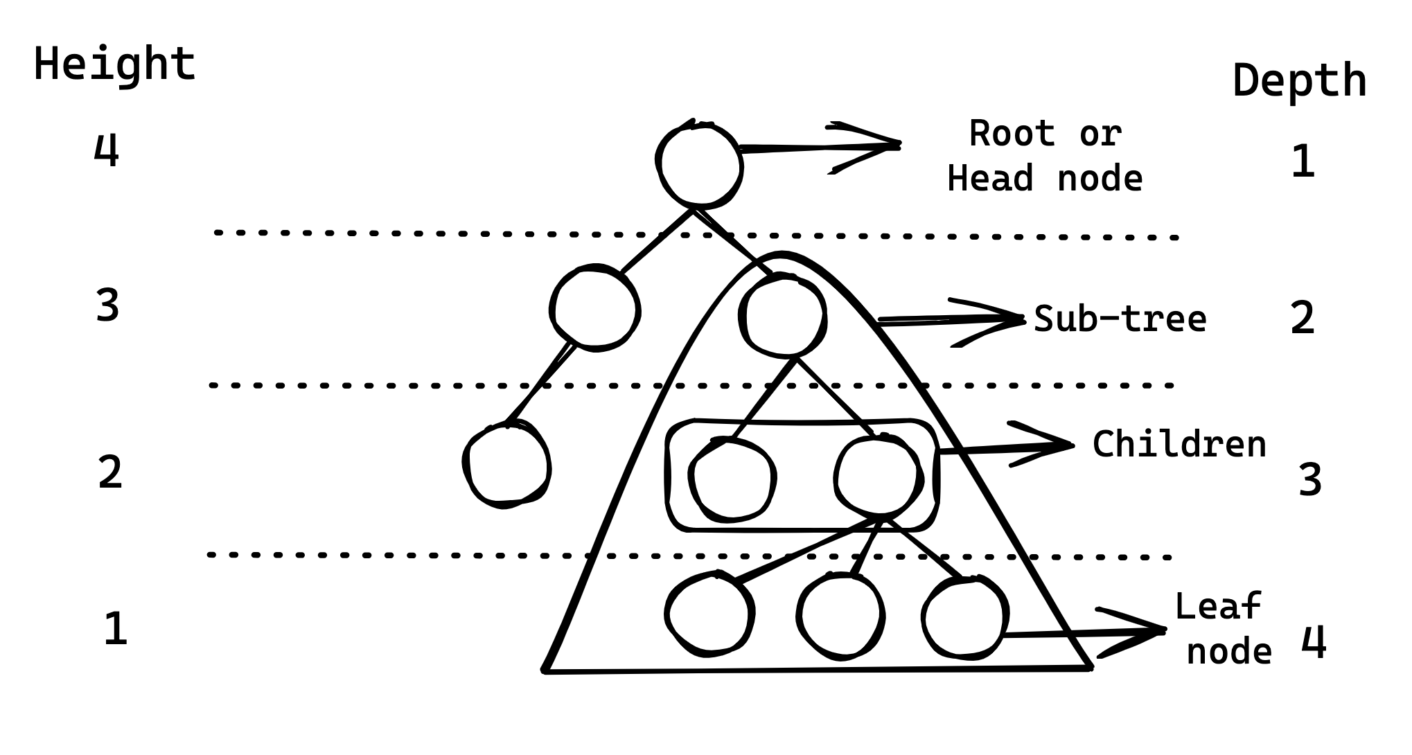
A tree containing nodes with a maximum of n children can be called an n-ary tree. This article covers the case where n = 2: the binary tree. In particular a special type of binary tree, called the binary search tree, which enforces a specific ordering on its nodes will be investigated.
What are binary search trees?
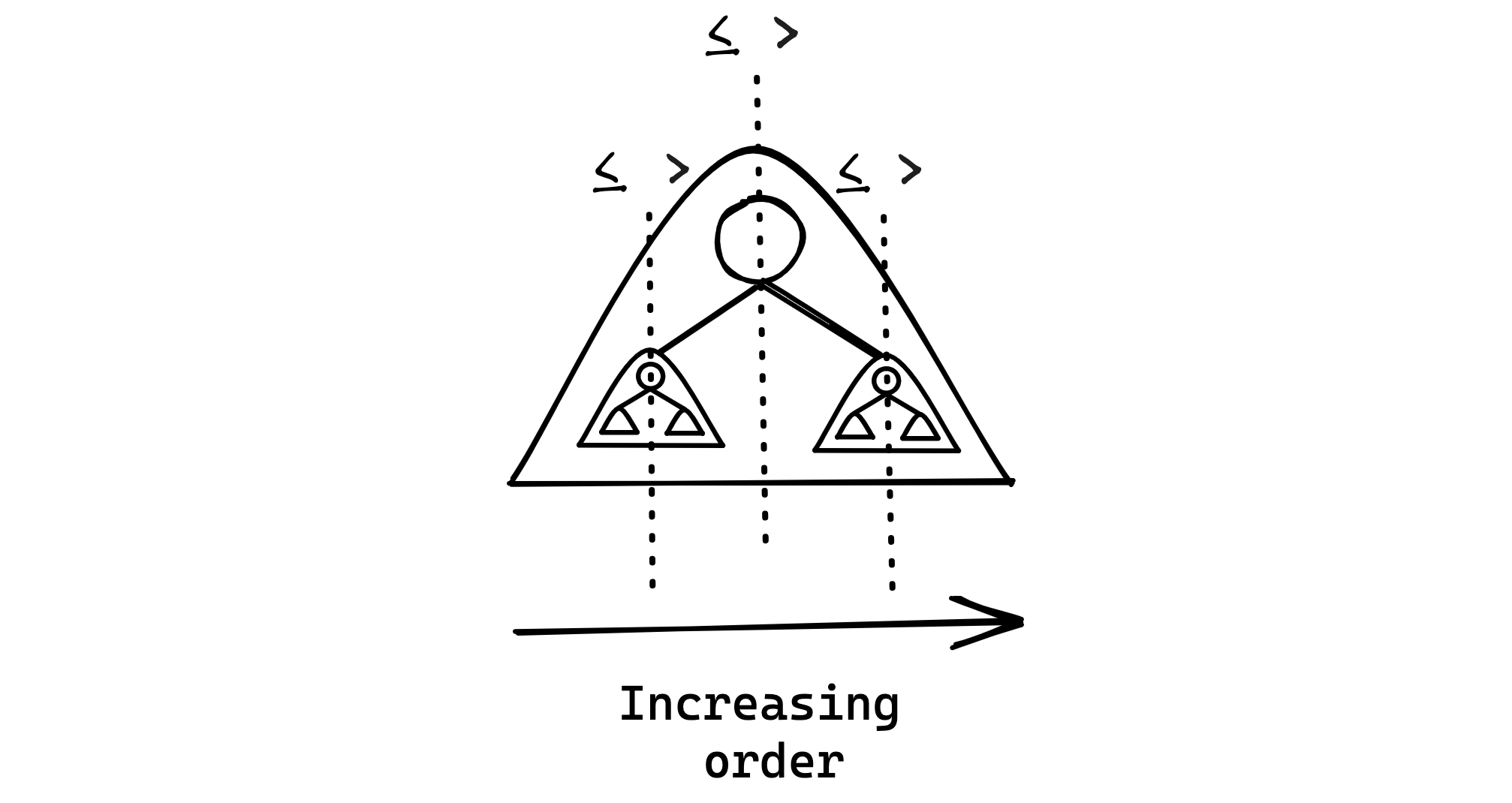
Binary search trees enforce the ‘binary search invariant’: given a key and a comparator function, every node in the left sub-tree of its parent node has a key that is $\le$ to the parent node’s key, and conversely every key in the right sub-tree is $>$ than the parent’s key. The below diagram provides visual intuition of this concept:
Implementations of binary search trees
The most common implementation of binary search trees is the linked list implementation. However, as an exercise in understanding the concept space efficiency, the array implementation is also considered. Code will be written in Python. All code is also available on my github.
Array implementation:
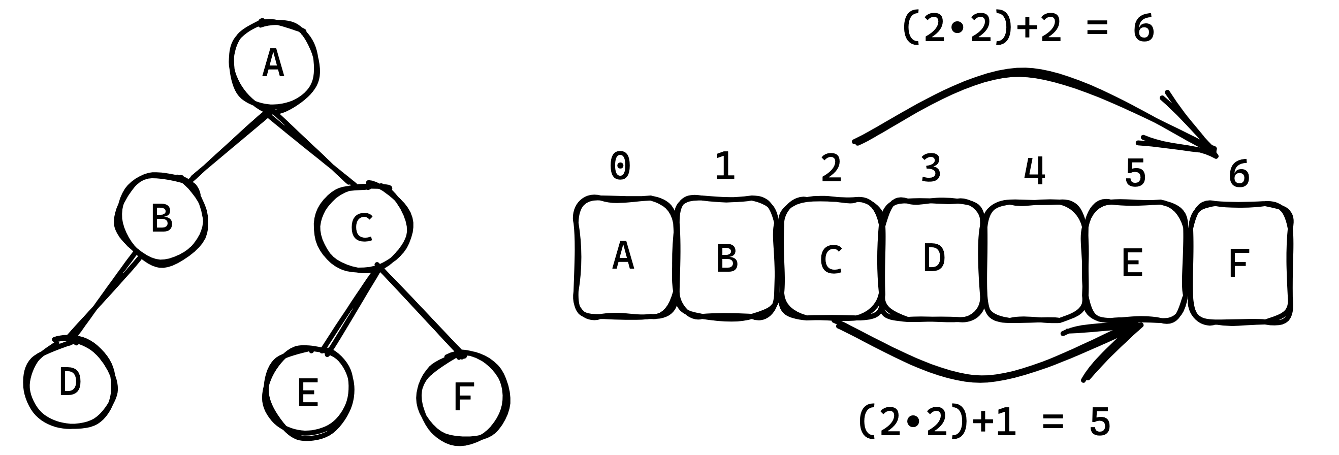
This implementation stores the binary search tree as an array of nodes where indices delineate the relationship between the nodes. Specifically for a node at index $i$, its left child is at index $2i+1$ and its right child is at index $2i+2$. The below diagram visually describes this concept:
Provided below is the node class used in this implementation:
class Node:
    def __init__(self,Value) -> None:
        self.Value = Value

    def __str__(self) -> str:
        return str(self.Value)

    __repr__ = __str__
The str() method was overwritten to make console outputs meaningful. The repr() was also overwritten as python calls this method when printing out objects in an iterable. This ensures that outputs look like:
[3 2 5 None None None 7 None None None None None None 6 9]
Rather than:
[<Node.Node object at 0x1086fc290> <Node.Node object at 0x1086fcb50>
 <Node.Node object at 0x108b22590> None None None
 <Node.Node object at 0x1086fc310> None None None None None None
 <Node.Node object at 0x1086fcc90> <Node.Node object at 0x1087224d0>]
Using this node class and above discussed indexing, the BinaryTree class can now be implemented. As python does not have the concept of a fixed size array, the NumPy package must be imported. Provided below are the necessary imports and init method of the class:
from Node import Node
import numpy as np
import sys
np.set_printoptions(threshold=sys.maxsize)

class BinaryTree:
    def __init__(self) -> None:
        self.Tree = np.empty(1, dtype=Node)
On initialization, the BinaryTree object is instantiated with an empty array of type Node and length = 1.
Now the insert method can be defined:
def Insert(self, ValueToInsert) -> None:
    # Handle case where tree is empty,
    # ie. there is no headnode
    if self.Tree[0] == None:
        self.Tree[0] = Node(ValueToInsert)
    else:
        # Start comparing values from the headnode
        CurrentNode = self.Tree[0]
        Inserted = False
        Index = 0
        while Inserted == False:
            # Check if new level has to be created
            if len(self.Tree) <= (2*Index)+1:
                NewTree = np.empty(2*len(self.Tree)+1, dtype=Node)
                for i, j in np.ndenumerate(self.Tree):
                    NewTree[i] = j
                self.Tree = NewTree
            # Insert node if necessary index is not none or
            # update index and currentnode and continue search
            if (ValueToInsert > CurrentNode.Value and
                self.Tree[(2*Index)+2] == None):
                self.Tree[(2*Index)+2] = Node(ValueToInsert)
                Inserted = True
            elif (ValueToInsert <= CurrentNode.Value and
                  self.Tree[(2*Index)+1] == None):
                self.Tree[(2*Index)+1] = Node(ValueToInsert)
                Inserted = True
            elif (ValueToInsert > CurrentNode.Value and
                  self.Tree[(2*Index)+2] != None):
                CurrentNode = self.Tree[(2*Index)+2]
                Index = ((2*Index)+2)
            elif (ValueToInsert <= CurrentNode.Value and
                  self.Tree[(2*Index)+1] != None):
                CurrentNode = self.Tree[(2*Index)+1]
                Index = ((2*Index)+1)
The method first checks if the tree is empty (ie., if the headnode is None). If so, the headnode is set to be a node of ValueToInsert.
If the tree is not empty, the method begins comparing values - starting with the headnode - by entering a while loop that continues until the value has been inserted.
Inside the while loop, the method first checks if a new level has to be created in the tree. This is necessary if the node is not yet inserted, and the array does not have capacity to store nodes deeper than CurrentNode. Inserted being false implies the need for indices at $(2 \cdot \operatorname{Index})+1$ (if ValueToInsert is to be the left child of CurrentNode) or $(2 \cdot \operatorname{Index})+2$ (if ValueToInsert is to be the right child of CurrentNode). As the loop only runs when this condition is met, and $(2 \cdot \operatorname{Index})+1 < (2 \cdot \operatorname{Index})+2$, it is sufficient to check if the length of the tree array is $<(2 \cdot \operatorname{Index})+1$. In the case that this is true, a new level must be created.
To create a new level, a NewTree array of size $2\cdot\operatorname{len(self.Tree)}+1$ must be created and all the values from the previous array must inserted into this new array. The new size is set to $2\cdot\operatorname{len(self.Tree)}+1$ due to the exponential nature of tree growth.
The method then checks if it can insert the new node by checking four conditions. If ValueToInsert is greater than, or less than or equal to the value of the current node and the right or left child is None, it creates a new Node and assigns it to the right or left child. If the right or left child is not None, it updates CurrentNode and Index to point to the right or left child and continues with the next iteration of the while loop.
Pitfalls of the array implementation:
Now that the insert method is defined, memory efficiency problems of the array implementation become clear. Consider the below code to create a BinaryTree object, insert values and print the resulting array:
Tree = BinaryTree()
Tree.Insert(10)
Tree.Insert(12)
Tree.Insert(8)
Tree.Insert(16)
Tree.Insert(14)
Tree.Insert(5)
Tree.Insert(6)
Tree.Insert(7)
Tree.Insert(3)
Tree.Insert(11)
print(Tree.Tree)
It outputs:
[10 8 12 5 None 11 16 3 6 None None None None 14 None None None None 7
 None None None None None None None None None None None None]
It is immediately evident from the number of ‘None’ values that the size of the array generated is significantly larger than the size of the input. In this case, to insert 10 values, an array of size 31 was created. However, this is not the worst case. Consider inserting values in an ascending order to the tree:
Tree = BinaryTree()
for i in range(6):
    Tree.Insert(i)
print(Tree.Tree)
This code outputs:
[0 None 1 None None None 2 None None None None None None None 3 None None
 None None None None None None None None None None None None None 4 None
 None None None None None None None None None None None None None None
 None None None None None None None None None None None None None None
 None None 5]
To insert 6 values, an array of size 63 was created. More generally, for a tree of $n$ nodes, a tight upper bound on the size of the necessary array ($S_a$) is:
$$S_a \le 2^{n}-1$$
Hence, in the worst case, space exponential in the number of nodes inserted is necessary. This is clearly inefficient. In terms of big-O notation, it can be said that the array implementation has a space complexity of $O(2^{n})$. The linked list implementation addresses this issue.
Linked list implementation:
This implementation stores the binary search tree as a special type of linked list where each node has pointers to its left and right child. Provided below is the code for the node class:
class Node:
    def __init__(self,Value,LeftNode=None,RightNode=None) -> None:
        self.Value = Value
        self.LeftNode = LeftNode
        self.RightNode = RightNode
The initializer for the node class allows instantiating node objects with LeftNode and RightNode. In the absence of this they default to None.
Using this, the BinaryTree class can now be written:
from Node import Node
class BinaryTree:
    def __init__(self) -> None:
        self.HeadNode = None
As an iterative implementation of insert was already covered in the previous array implementation, a recursive version will be implemented here. Given below is code for the recursive insert:
def RecursiveInsert(self, ValueToInsert: int, Subtree=None):
    # Handle case where tree is emptry,
    # ie. headnode is none
    if self.HeadNode == None:
        self.HeadNode = Node(ValueToInsert)
    else:
        if Subtree == None:
            Subtree = self.HeadNode
        if ValueToInsert > Subtree.Value and Subtree.RightNode != None:
            self.RecursiveInsert(ValueToInsert, Subtree.RightNode)
        elif ValueToInsert <= Subtree.Value and Subtree.LeftNode != None:
            self.RecursiveInsert(ValueToInsert, Subtree.LeftNode)
        if ValueToInsert > Subtree.Value and Subtree.RightNode == None:
            Subtree.RightNode = Node(ValueToInsert)
        elif ValueToInsert <= Subtree.Value and Subtree.LeftNode == None:
            Subtree.LeftNode = Node(ValueToInsert)
This insert works by utilizing the tree-subtree relationship. If the tree is populated, it first considers the entire tree by starting with the headnode. Depending on the key of the node to be inserted, the function then calls itself on the left or the right child. This child and its children also form an equal valid tree. Therefore, this process can be repeated, and is repeated until a suitable position for the node to be insert is found. This method can best be described diagrammatically:
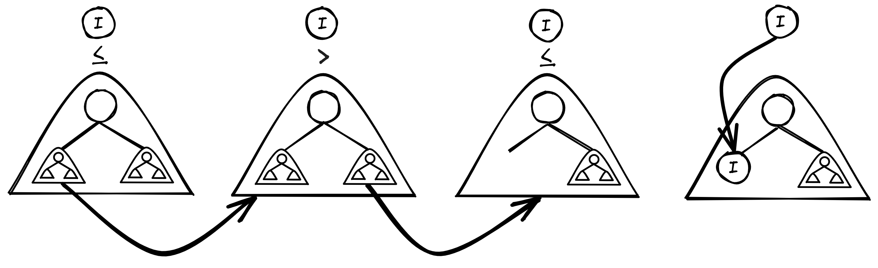
Where the above diagram describes a process that is equivalent to the below iterative comparison:

In this manner, the linked list implementation lends itself to simple exploitation of the recursive nature of trees.
A primary strength of the binary search tree is the efficiency of its search time. Given below is code for the search method:
def Search(self, ValueToBeFound) -> Node | None:
    if self.HeadNode == None:
        return None
    else:
        CurrentNode = self.HeadNode
        EndReached = False
        ReturnNode = None
        while EndReached == False:
            if ValueToBeFound > CurrentNode.Value and CurrentNode.RightNode != None:
                CurrentNode = CurrentNode.RightNode
            elif ValueToBeFound < CurrentNode.Value and CurrentNode.LeftNode != None:
                CurrentNode = CurrentNode.LeftNode
            elif ((ValueToBeFound > CurrentNode.Value and CurrentNode.RightNode == None) or
                  (ValueToBeFound < CurrentNode.Value and CurrentNode.LeftNode == None)):
                EndReached = True
            elif CurrentNode.Value == ValueToBeFound:
                ReturnNode = CurrentNode
                EndReached = True
        return ReturnNode
The search method utilizes the ordering in the binary search tree to its advantage. If the ValueToBeFound is greater than the value of the CurrentNode and the CurrentNode has a right node, CurrentNode is set to CurrentNode.RightNode. Conversely, if the ValueToBeFound is lesser than the value of the CurrentNode and the CurrentNode has a left node, CurrentNode is set to CurrentNode.LeftNode. While in this process, if a situation arises such that the ValueToBeFound is not equal to the value of the CurrentNode and the CurrentNode does not possess the necessary left/right child, the value is not in the tree and the search returns None. In the case that the value of the current node is the ValueToBeFound, CurrentNode is returned.
Analyzing the efficiency of the search method
Best case: The balanced binary search tree
Consider a ‘balanced’ binary search tree as depicted below:

We can define a ‘balanced’ tree to be one such that the deepest nodes of any two branches of the tree do not differ by a height of more than 1. In other words: the binary search tree is as ‘filled’ as possible. In such a case, the number of operations necessary to search a balanced tree of $n$ nodes for a specific node (as defined by the number of nodes required to traverse before reaching the desired node) $N_o$, would be of the form:
$$N_o \le a\log_2(n)-b$$
In other words, the best case time complexity of the search operation of a binary search tree of $n$ nodes can be written as $\Omega(log_2(n))$. Such search time is highly efficient and is one of the primary advantages of the binary search tree.
Worst case: The degenerate binary search tree
In the worst case, that is if nodes are inserted in an ascending or descending order with respect to its keys, the binary search tree devolves to a linked list. For better visualization, consider the case where nodes with keys of an ascending order are inserted:
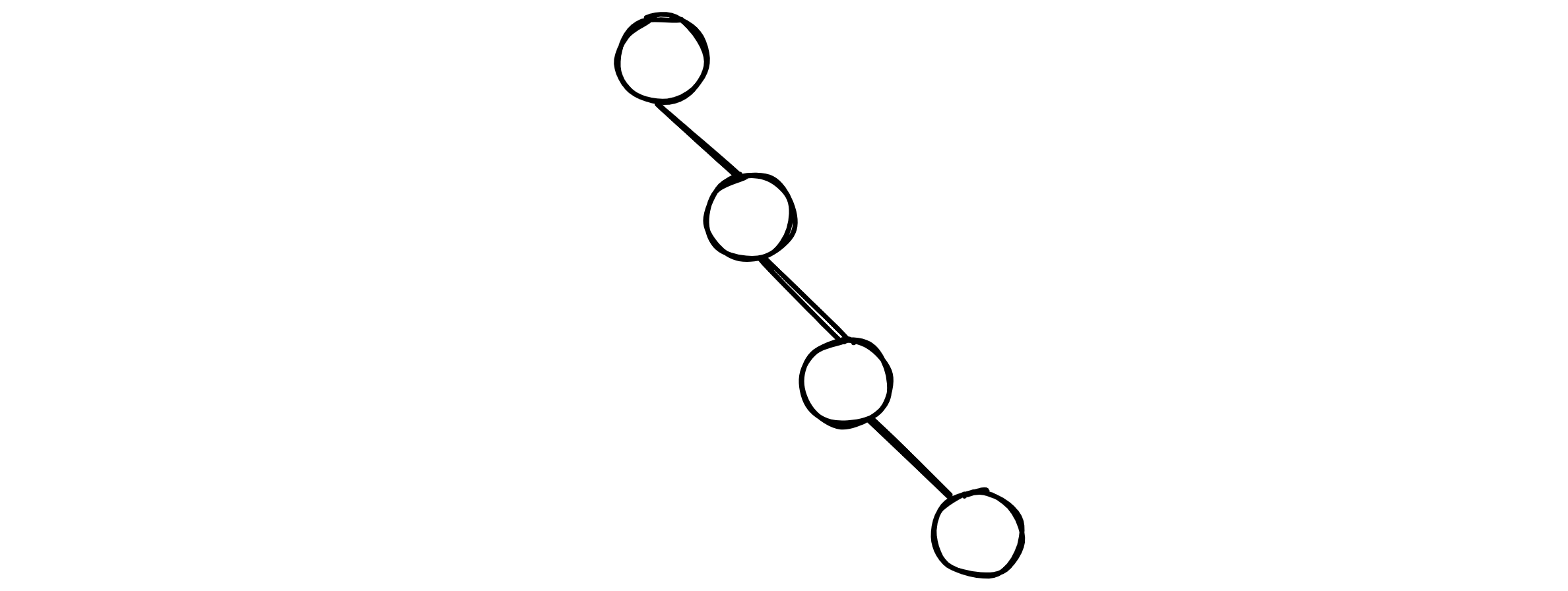
In this case, by similar analysis as in the above case, the worst case time complexity of the search operation of a binary search tree can be written as $O(n)$. This is significantly slower and defeats the prurpose of the tree structure.
AVL trees - correcting pitfalls of the binary search tree
To address this issue of the degenerate binary search tree, it would be desireable to create a tree data structure that can actively balance itself. That is, whenever a node is inserted, the tree can check for imbalances in its nodes and address them without breaking the binary search invariant. The oldest and most ‘strictly balanced’ of the self-balancing binary search trees is the AVl (Adelson-Velsky and Landis) tree. A key feature of this data structure is the concept of the ‘balance factor’ of a node $B_f(n)$ which is defined as:
$$B_f(n) = \operatorname{Height}(\operatorname{LeftSubtree}(n)) - \operatorname{Height}(\operatorname{RightSubtree}(n))$$
AVL trees enforce the AVL invariant, which states that:
$$|B_f(n)| \le 1$$
or alternatively:
$$B_f(n) \in -1,0,1 $$
This ensures that the tree remains balanced.
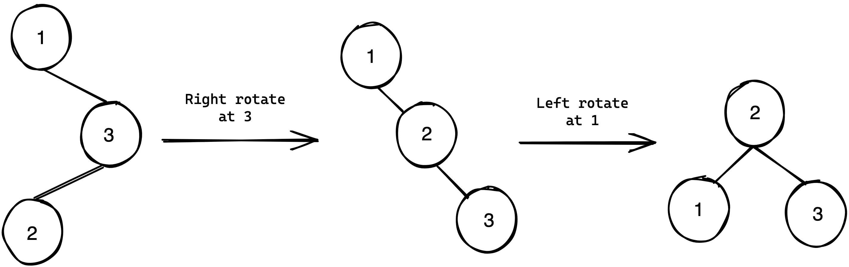
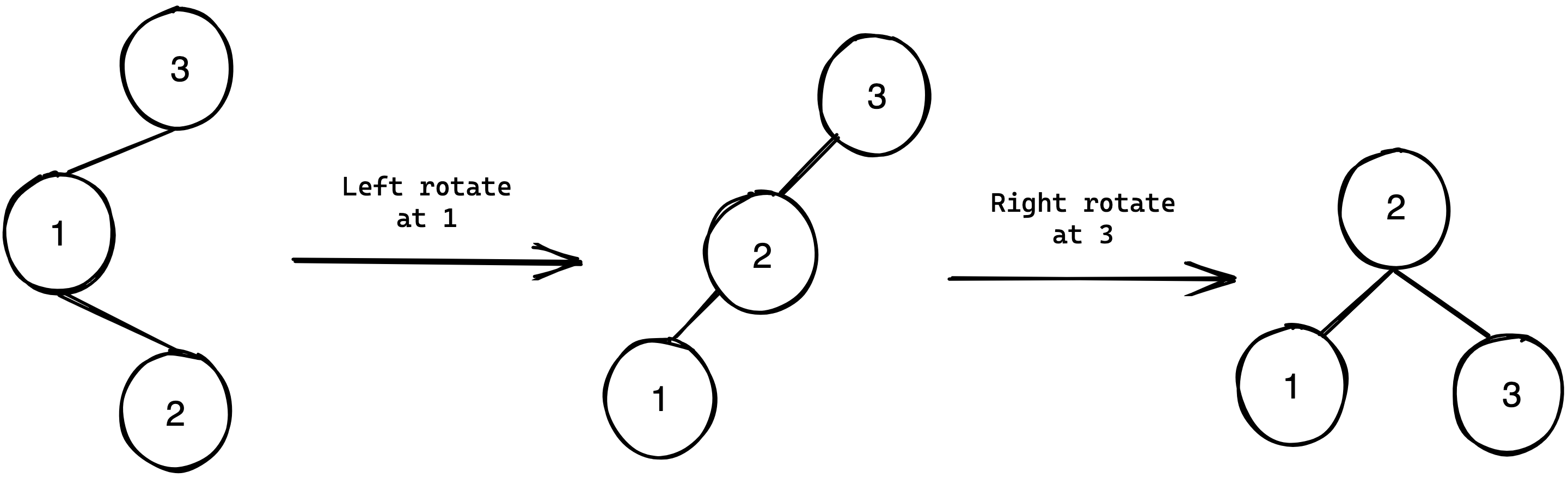
Another key feature are the left and right rotations. These rotations are transformations of the binary search tree that do not break the binary search invariant. The figure below best demonstrates this:
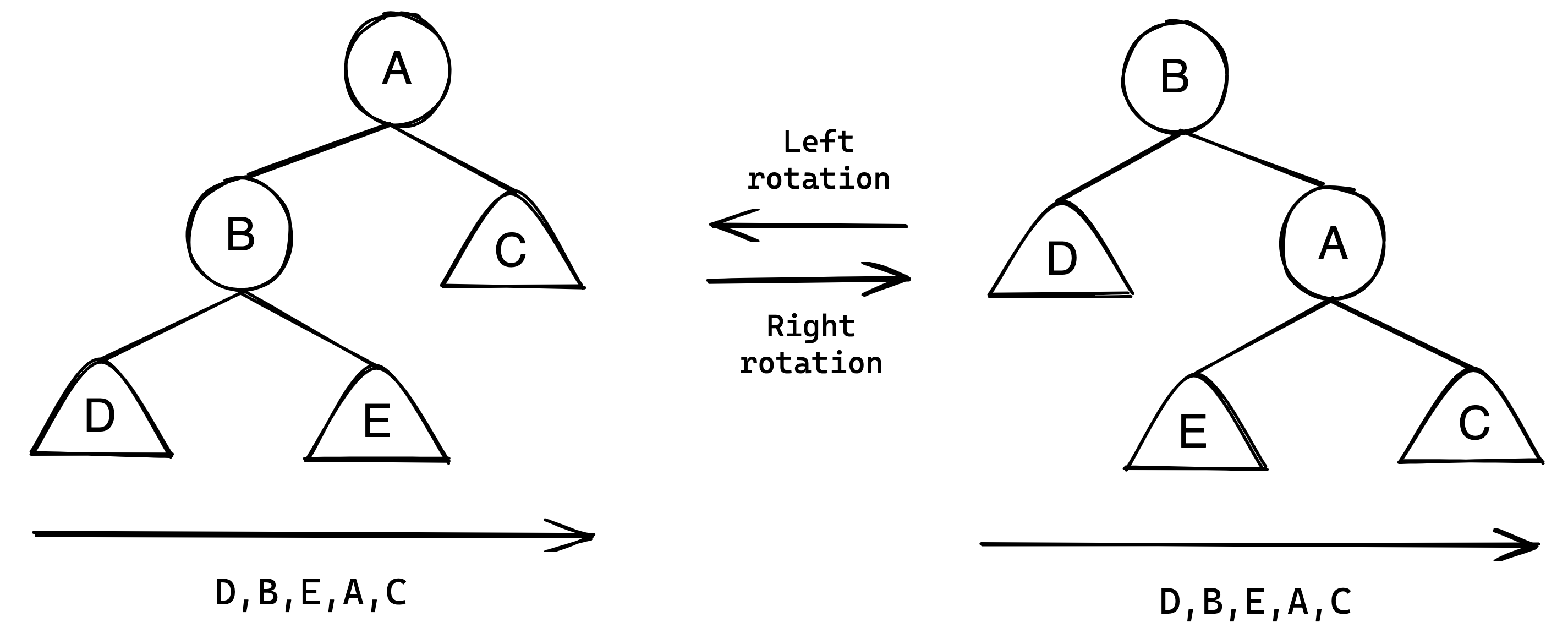
As the ascending (left to right) order of the tree does not change under the transformation, it does not break the binary search invariant. The application of these in balancing the binary tree are demonstrated by the below 4 cases:
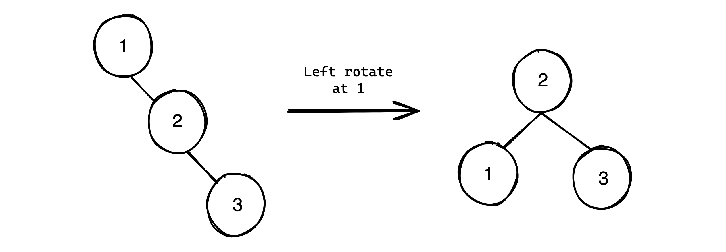
Left rotate
Right rotate
Right-Left rotate
Left-Right rotate
These cases encapsulate all combinations of imbalances that can be encountered in a binary search tree. To better understand this concept it is important to establish the idea of a node being ’left-skewed’ or ‘right-skewed’. Consider again the definition of the balance factor:
$$B_f(n) = \operatorname{Height}(\operatorname{LeftSubtree}(n)) - \operatorname{Height}(\operatorname{RightSubtree}(n))$$
If a node’s balance factor is negative, the height of it’s right subtree is larger than the height of it’s left subtree, and the node can be considered as ‘right-skewed’. Conversely If a node’s balance factor is positive, the height of it’s left subtree is larger than the height of it’s right subtree, and the node can be considered as ’left-skewed’.
Now consider the case of the left rotate. The conditions under which one must apply the left rotate can therefore be formulated as: “if a node is right-skewed and it’s right child is right-skewed, then apply the left rotate to it”. In similar fashion conditions for the other rotations can be formulated.
Using these concepts the AVL tree can now be implemented. As the each node now needs to have an associated height and a balance factor, the node class must be changed as below:
class Node:
    def __init__(self,Value,LeftNode=None,RightNode=None) -> None:
        self.Value = Value
        self.BalanceFactor = 0
        self.Height = 1
        self.LeftNode = LeftNode
        self.RightNode = RightNode
With the node class implemented, the AVLTree class can now be implemented:
from Node import Node
import copy
class AVLTree:
    def __init__(self) -> None:
        self.HeadNode = None
The ‘copy’ package is imported to implement the left and right rotations. Provided below is code for these:
def LeftRotate(self, Subtree: Node):
    print(f"L at {Subtree.Value} \n")
    Copy = copy.deepcopy(Subtree)
    RightNode = Copy.RightNode
    Copy.RightNode = RightNode.LeftNode
    RightNode.LeftNode = Copy
    Subtree.LeftNode = RightNode.LeftNode
    Subtree.RightNode = RightNode.RightNode
    Subtree.Value = RightNode.Value
    Subtree.Height = RightNode.Height

    Subtree.LeftNode.Height = 1 + max(self.GetHeight(Subtree.LeftNode.LeftNode), self.GetHeight(Subtree.LeftNode.RightNode))
    Subtree.Height = 1 + max(self.GetHeight(Subtree.LeftNode), self.GetHeight(Subtree.RightNode))


def RightRotate(self, Subtree: Node):
    print(f"R at {Subtree.Value} \n")
    Copy = copy.deepcopy(Subtree)
    LeftNode = Copy.LeftNode
    Copy.LeftNode = LeftNode.RightNode
    LeftNode.RightNode = Copy
    Subtree.LeftNode = LeftNode.LeftNode
    Subtree.RightNode = LeftNode.RightNode
    Subtree.Value = LeftNode.Value
    Subtree.Height = LeftNode.Height

    Subtree.RightNode.Height = 1 + max(self.GetHeight(Subtree.RightNode.LeftNode), self.GetHeight(Subtree.RightNode.RightNode))
    Subtree.Height = 1 + max(self.GetHeight(Subtree.LeftNode), self.GetHeight(Subtree.RightNode))
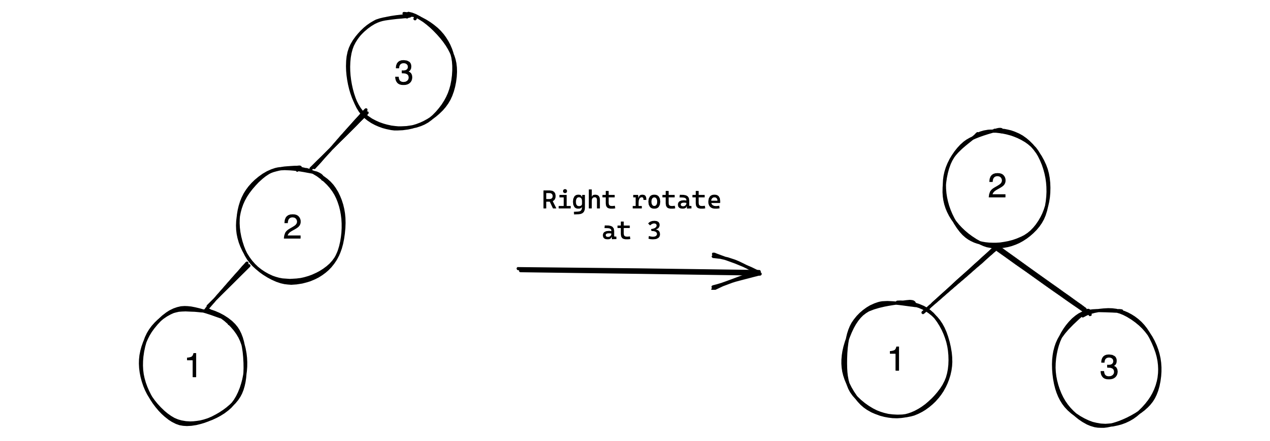
The diagram below describes RightRotate:
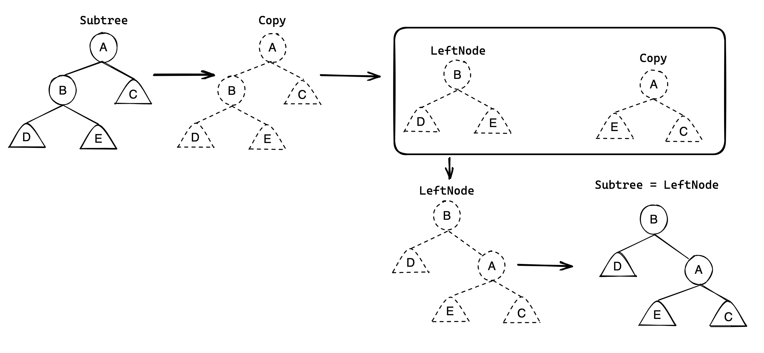
LeftRotate functions analogous to this.
Alongside these, helper functions to handle null cases must be implemented:
#To handle null values

def GetLeftChild(self, Node: Node):
    if Node == None:
        return None
    else:
        return Node.LeftNode


def GetRightChild(self, Node: Node):
    if Node == None:
        return None
    else:
        return Node.RightNode


def GetHeight(self, Node: Node):
    if Node == None:
        return 0
    return Node.Height


def GetBalance(self, Node: Node):
    if Node == None:
        return 0
    return self.GetHeight(Node.LeftNode) - self.GetHeight(Node.RightNode)
Now the insert function can be implemented. This function also ensures that the tree remains balanced ie. maintains the AVL invariant. That is, the insert function balances out any imbalances introduced by inserting a node into the tree. To do so, it is necessary to know all the nodes traversed when inserting a node, and to be able to access them in a ’leaf up’ fashion. This can be iteratively done using a stack data structure to store all nodes visited. Alternatively, one can take advantage of the call stack with a recursive implementation to keep track of and visit all traversed nodes in the desired order. The latter is implemented in the below function:
def RecursiveInsert(self, ValueToInsert: int, Subtree=None):
    if self.HeadNode == None:
        self.HeadNode = Node(ValueToInsert)
        self.HeadNode.Height = 1 + max(self.GetHeight(self.HeadNode.LeftNode),self.GetHeight(self.HeadNode.RightNode))
        self.HeadNode.BalanceFactor = self.GetBalance(Subtree)
    else:
        if Subtree == None:
            Subtree = self.HeadNode
        if ValueToInsert > Subtree.Value and Subtree.RightNode != None:
            self.RecursiveInsert(ValueToInsert, Subtree.RightNode)
        elif ValueToInsert <= Subtree.Value and Subtree.LeftNode != None:
            self.RecursiveInsert(ValueToInsert, Subtree.LeftNode)
        if ValueToInsert > Subtree.Value and Subtree.RightNode == None:
            Subtree.RightNode = Node(ValueToInsert)
        elif ValueToInsert <= Subtree.Value and Subtree.LeftNode == None:
            Subtree.LeftNode = Node(ValueToInsert)

        Subtree.Height = 1 + max(self.GetHeight(Subtree.LeftNode),self.GetHeight(Subtree.RightNode))

        Subtree.BalanceFactor = self.GetBalance(Subtree)

        # If Subtree.BalanceFactor -ve, right skewed
        # If Subtree.BalanceFactor +ve, left skewed

        # Node is left-skewed and it’s left child is right-skewed
        if Subtree.BalanceFactor > 1 and self.GetHeight(self.GetLeftChild(Subtree.LeftNode)) <= self.GetHeight(self.GetRightChild(Subtree.LeftNode)):
            LeftNode = Subtree.LeftNode
            self.LeftRotate(LeftNode)
            self.RightRotate(Subtree)
        # Node is left-skewed and it’s left child is left-skewed
        elif Subtree.BalanceFactor > 1 and self.GetHeight(self.GetLeftChild(Subtree.LeftNode)) > self.GetHeight(self.GetRightChild(Subtree.LeftNode)):
            self.RightRotate(Subtree)
        # Node is right-skewed and it’s right child is left-skewed
        elif Subtree.BalanceFactor < -1 and self.GetHeight(self.GetLeftChild(Subtree.RightNode)) > self.GetHeight(self.GetRightChild(Subtree.RightNode)):
            RightNode = Subtree.RightNode
            self.RightRotate(RightNode)
            self.LeftRotate(Subtree)
        # Node is right-skewed and it’s right child is right-skewed
        elif Subtree.BalanceFactor < -1 and self.GetHeight(self.GetLeftChild(Subtree.RightNode)) < self.GetHeight(self.GetRightChild(Subtree.RightNode)):
            self.LeftRotate(Subtree)
This insert function first fully implements the previously investigated recursive insert. Hence, the insertion component is effectively done once the ValueToInsert is set as a suitable node’s left or right child. Then, the function updates the node’s height and its balance factor. After this, it checks for the four scenarios that were discussed above and carries out rotations as necessary. After carrying out the necessary checks and rotations, the function is complete, and the call-stack is popped. Hence, execution is resumed on the node’s parent to again carry out the necessary checks and rotations. In this manner, the height of every node traversed is updated, their balance factor is checked, and the necessary rotations are carried out to ensure that the binary search tree remains balanced.
AVL tree in action
Finally, now that the insert function is implemented, utility of the AVL tree can be investigated using the below printTree() function obtained from the internet:
def printTree(node:Node, level=0):
    if node != None:
        printTree(node.LeftNode, level + 1)
        print(' ' * 4 * level + '-> ' + str(node.Value))
        printTree(node.RightNode, level + 1)
Consider the below code and its output:
Tree = BinaryTree()
for i in  range(10):
     Tree.Insert(i)

printTree(Tree.HeadNode)
-> 0
    -> 1
        -> 2
            -> 3
                -> 4
                    -> 5
                        -> 6
                            -> 7
                                -> 8
                                    -> 9
Contrast this against the same insertions carried out on an AVL tree:
Tree = AVLTree()
for i in  range(10):
     Tree.RecursiveInsert(i)

printTree(Tree.HeadNode)
L at 0

L at 2

L at 1

L at 4

L at 6

L at 5

        -> 0
    -> 1
        -> 2
-> 3
            -> 4
        -> 5
            -> 6
    -> 7
        -> 8
            -> 9
It is evident that the AVL invariant ensures that tree height, and thereby search time, is minimized. To demonstrate functionality of all the various combinations of rotations, code to insert 10 random values $\in [1,100]$ and its output(s) is given:
import random
Tree = AVLTree()

for i in range(10):
    j = random.randint(1,100)
    Tree.RecursiveInsert(j)

printTree(Tree.HeadNode)
R at 64

R at 99

L at 64

L at 3

R at 62

        -> 3
    -> 57
            -> 61
        -> 61
            -> 62
-> 63
        -> 64
            -> 69
    -> 73
        -> 99
L at 1

R at 43

R at 10

L at 1

R at 82

L at 43

R at 82

        -> 1
    -> 3
        -> 10
-> 32
        -> 43
            -> 45
    -> 62
            -> 64
        -> 82
            -> 82
Analysing the search efficiency of the AVL tree:
AVL trees ensure a search time of $O(\log(n))$. A proof of this is given below:
The minimum number of nodes required to form an AVL tree of a desired height can be given by the recursive relation:
$$m(h) = 1 + m(h-1) + m(h-2)$$
With the base case:
$$m(1) = 1$$
$$m(2) = 2$$
As $m(h)$ is strictly increasing,
$$m(h-1)>m(h-2)$$
Therefore, the below inequality holds:
$$1+m(h-1)>m(h-2)$$
$$1+m(h-1)+m(h-2)>2m(h-2)$$
$$m(h)>2m(h-2)$$
By repeatedly applying this argument:
$$m(h)>2m(h-2)>4m(h-4)>8m(h-6)…$$
$$m(h)>2^{i}m(h-2i)$$
As the base case $m(1)=1$ is known, solve for $i$ such that $m(h-2i) = m(1)$
$$i = \frac{h-1}{2}$$
Therefore,
$$m(h)>2^{\frac{h-1}{2}}m(1)$$
$$m(h)>2^{\frac{h-1}{2}}$$
$$\log_2{m(h)}>\frac{h-1}{2}$$
$$2\log_2{m(h)}>h-1$$
$$2\log_2{m(h)}+1>h$$
Hence, an upper bound on the height of an AVL tree is:
$$h<2\log_2{m(h)}+1$$
By the definition of $m(h)$,
$$m(h) \le n(h)$$
Where $n(h)$ is the actual number of nodes at a specific height. Therefore,
$$2\log_2{m(h)}+1 \le 2\log_2{n(h)}+1$$
Hence:
$$h<2\log_2{n(h)}+1$$
Therefore, for a tree of $n$ nodes, an upper bound on its height can be written as:
$$h<2\log_2{n}+1$$
This upper bound on height also provides an upper bound on the number of nodes required to traverse before reaching the leaf node. Hence, as the number of operations necessary to search a balanced tree of $n$ nodes for a specific node: $N_o$ is defined by the number of nodes required to traverse before reaching the desired node,
$$N_o<2\log_2{n}+1$$
Hence, AVL trees ensure a worst case search time of $O(\log(n))$
QED