Hash table
Hash tables, in their basic implementation, are a linear data structure.

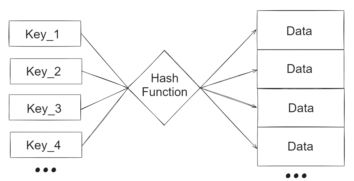
Fundamentally, hash tables are built on top of arrays. Given data that can be expressed as a key value pair, a hash table hashes the key to its “unique” corresponding index and stores the data at that index.
Hash functions
Assume that the set of keys $K$ being dealt with are either integers or are more generally some set of values with integer mapping $f:K \to \mathbb{Z} \text{ }$ (note this $f$ may not be injective, problems start here). A hash is a function $h: \mathbb{Z} \to M$ where $M$ is the set of all memory locations such that $h$ is surjective. $h$ is not considered a bijection because computers have finite memory. This will have implications, called collisions, that will be dealt with later in the article.
An example hash function would be:
$$h(k) = k \text{ mod } m$$
Where $m$ is the total number of memory locations available.
Naive implementation of a hash table
Here by naive implementation it is meant that the hash table ignores the surjective nature of the hash function. The below code will be written in python. All code is available on github.
The key-value representation of the data is captured by the Node class:
class Node:
    def __init__(self,Key,Data) -> None:
        self.Key = Key
        self.Data = Data

    def __str__(self) -> str:
        return f"({self.Key}, {self.Data})"

    __repr__ = __str__
The keyspace here is assumed strings of length 5.
Next we define the methods of the HashTable class. The underlying array is of size 10. Of foremost importance would be definition of the hash function:
$$h(k) = k \text{ mod } m$$
def Hash(self,Key):
    IntRep = 0
    for Char in Key:
        IntRep += ord(Char)
    Index = IntRep%10
    return Index
The hash function defined is very rudimentary. Outside of the obvious way collisions can occur, through the cyclic nature of modulo, another weakness to be noted is that the process of converting the string to its integer representation is itself not injective. For example, “jrptf” and “jrhmu” have the same integer representation and therefore the same hash.
The other functions are fairly straightforward:
def Insert(self,Node:Node):
    Index = self.Hash(Node.Key)
    self.Table[Index] = Node

def Delete(self,Key):
    Index = self.Hash(Key)
    self.Table[Index] = None

def Find(self,Key):
    Index = self.Hash(Key)
    return self.Table[Index]
Clearly all of these functions have constant $O(1)$ time complexity, as the hash function has constant time complexity for all fixed length strings and array reads and writes have constant time complexity. This is one of the major advantages of a hash table. To demonstrate collision issues, consider the below:
from HashTable import HashTable
from Node import Node

Table = HashTable()

Node1 = Node("jrptf",1314)
Node2 = Node("xyovo",4673)
Node3 = Node("xqoao",3566)
Node4 = Node("psiwf",2453)
Node5 = Node("szccc",9203)
Node6 = Node("pwnjl",3892)
Node7 = Node("wiink",1234)
Node8 = Node("krffq",5685)
Node9 = Node("pxawo",7722)
Node10 = Node("wtdmi",1231)

Table.Insert(Node1)
Table.Insert(Node2)
Table.Insert(Node3)
Table.Insert(Node4)
Table.Insert(Node5)
Table.Insert(Node6)
Table.Insert(Node7)
Table.Insert(Node8)
Table.Insert(Node9)
Table.Insert(Node10)

print(Table.Table)
Which outputs:
[(jrptf, 1314) (xyovo, 4673) (xqoao, 3566) (psiwf, 2453) (szccc, 9203)
 (pwnjl, 3892) (wiink, 1234) None (krffq, 5685) (wtdmi, 1231)]
Even though there were equivalent number of records to store as there was memory available, the record (“pxawo”,7722) was not stored. This is because there is a key collision between “pxawo” and “wtdmi”. This is an obvious flaw with the current implementation of the hash table.
Hash table with probing
Probing is a method of collision resolution. To achieve this the probing function is modified to be:

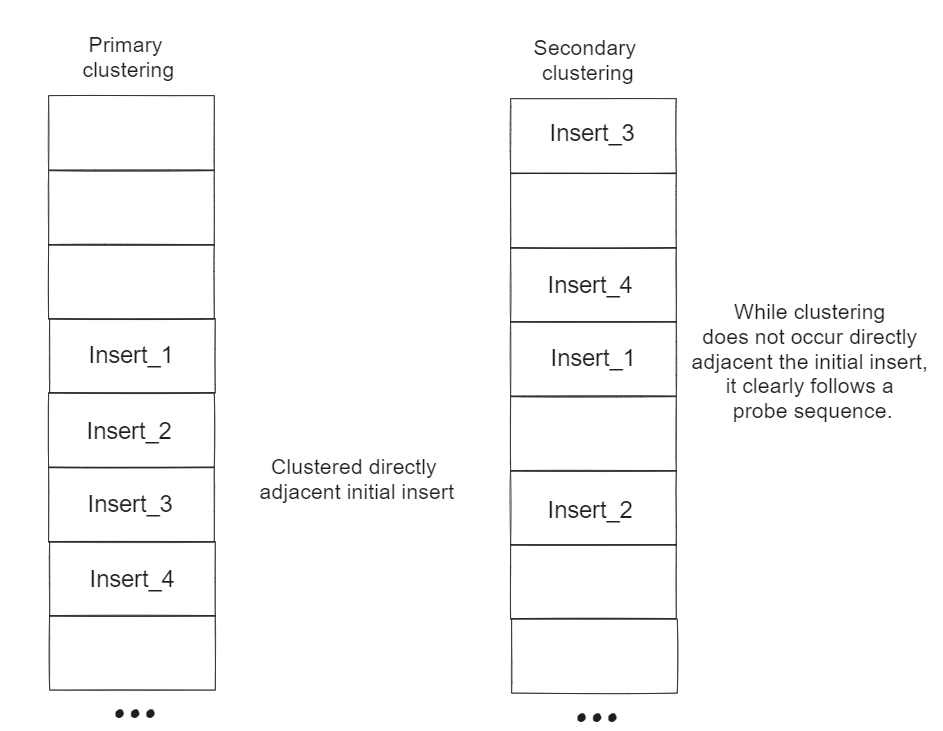
Where $A$ and $B$ are some constants. If $B \neq 0$, then the above hash function is called a quadratic probe. If $B = 0$, then the hash function devolves to a linear probe. While both of these methods resolve collisions, they cost added overhead when collisions are encountered. For all operations the worst case, that is when all keys for insertion will collide, time complexity is linear $O(n)$ in the number of records previously inserted. It must be kept in mind however that this is the worst case and probing is indeed an effective method of hash resolution generally. Quadratic probing does provide some benefits to linear probes in terms of preventing primary clustering. Below the types of clustering are pictorially described:

Given below is the python code for the modified hash function:
The other methods of the HashTable class were also modified:
Hash table with linked list chaining
Chaining is another common way to prevent collisions. In general, chaining involves nesting another data structure within the hash table to manage the collisions. Clearly, the worst case time complexity would devolve to that of the nested data structure. This section discusses linked list chaining.
Below is a simple implementation of a linked list:
from Node import Node

class LinkedList:
    def __init__(self) -> None:
        self.HeadNode = None

    def Insert(self,NodeToInsert:Node):
        NodeToInsert.Next = self.HeadNode
        self.HeadNode = NodeToInsert

    def Search(self,Key):
        CurrentNode = self.HeadNode
        while CurrentNode != None and CurrentNode.Key != Key:
            CurrentNode = CurrentNode.Next
        return CurrentNode

    def printSelf(self):
        CurrentNode = self.HeadNode
        Output = ""
        while CurrentNode.Next != None:
            Output = Output + f"{CurrentNode} -> "
            CurrentNode = CurrentNode.Next
        Output = Output + f"{CurrentNode}"
        print(Output)
When it comes to the HashTable class, the hash function remains unchanged. The other functions were modified to:
def Insert(self,Node:Node):
    Index = self.Hash(Node.Key)
    if self.Table[Index] == None:
        List = LinkedList()
        self.Table[Index] = List
    self.Table[Index].Insert(Node)

def Delete(self,Key):
    Index = self.Hash(Key)
    self.Table[Index] = None

def Find(self,Key):
    Index = self.Hash(Key)
    if self.Table[Index] == None:
        return None
    return self.Table[Index].Search(Key)